Introduction
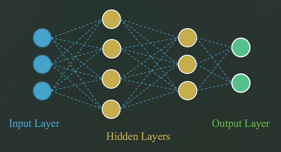
In the last few decades AI has undergone huge and rapid improvements, and one of its fastest growing fields is deep learning which falls under the machine learning category. In the same way, convolutional neural networks (CNNs) have improved dramatically over the past 10 years, going from few layers of depth to hundreds in some cases.
This blog post tries to give a technical insight on some of these CNNs and conducts a comparison between them on the task of classifying images of cats and dogs. For this purpose, firstly we will briefly discuss some of the available cloud GPU-enabled VMs providers, then dive into the classification and compare the accuracy of different CNN architectures for this task.
Choosing the right cloud service provider for the task
Currently there are many cloud service providers, but most of them do not offer GPU enabled machines. A simple search on the internet reveals some GPU-Enabled VMs providers. The top 3 candidates that we considered for our deep learning classification were Paperspace, Floydhub, and AWS. These providers offer per-hour billing options, which was one of the requirements for this showcase as we don’t need the instances for a longer period.
AWS seemed to offer good machine specs with reasonable prices (which vary depending on the server region), but unfortunately we were unable to provision any GPU enabled machines in EU or North America. The reason was that they have more demand than offer on their “On-Demand” machines, and the only solution for that is to buy a “reserved slot” which will cost thousands of dollars per month. For that reason we elected not to go with AWS.
FloydHub offered servers only in USA, but we wanted to go with EU located servers in compliance of EUs data protection regulations. For that reason we abandoned the idea of using their services. It is noted that in near future they are planning to provision EU located servers.
At the end Paperspace was the provider of choice for many reasons; they have very good pricing models and multiple ways to control expenses. Also, their machines specs are excellent for general machine learning or gaming purposes. They also provide VM templates that come bundled with standard Machine Learning backends like Keras, Tensorflow, CUDA, and others. That being said, those ML-in-a-Box machines might not be plug and play in some cases. In our case we had to change the versions of some of the bundled software to fix compatibility issues between Tensorflow, the machines CPU, and the machines’ GPU Drivers. This process is described in details in another Blog Post.
Environment & Networks
We are using Keras (V 2.2.0) with Tensorflow (V 1.5) backend to conduct this comparison on a GPU enabled machine (P5000) that is provided by the cloud VM provider “Paperspace”. Machine specifications can be found in “Machine Specs” section below. We also reverted to CUDA (V 9.0) for compatibility issues with Tensorflow (Versions 1.5 and later).
With this setup we were able to train 10 Epochs of each network in only 01:15:30 hours.
Following is a list of the trained CNNs:
- DenseNet201: 20,242,984 parameters and 201 layers.
- DenseNet169: 14,307,880 parameters and 169 layers.
- DenseNet121: 8,062,504 parameters and 121 layers.
- Resnet50: 25,636,712 parameters and 168 layers.
- InceptionV3: 23,851,784 parameters and 159 layers
- InceptionResNetV2: 55,873,736 parameters and 572 layers.
- MobileNet: 4,253,864 parameters and 88 layers.
- MobileNetV2: 3,539,136 parameters.
Training Data
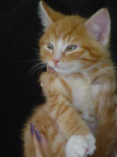
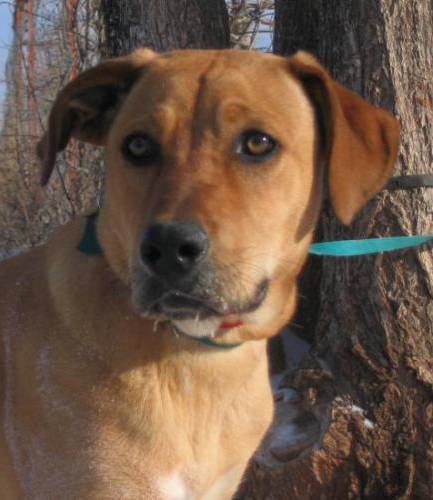
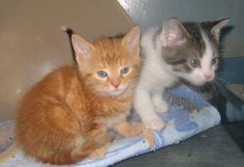
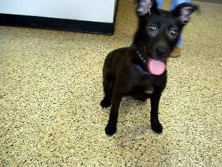
The training data comes from Kaggles’ cats vs dogs dataset. In our case, it consisted of 1000 cat images and 1000 dog images, with another 400 images each for validation.
A subset of images is used from each class in each epoch. Each image in that subset is subjected to augmentation techniques (rotating, channel shifting, zooming, shearing, flipping) to generate more data out of it. The resulting images are resized to (224*224 pixels) and feed into the input layer.
Below we can find a sample of the raw images before any augmentations and resizing.
Machine Specifications
The machine in use is a standard P5000 machine provided by Paperspace, the specs are as follows:
- MACHINE TYPE: P5000
- REGION: AMS1
- RAM: 30 GB
- CPUS: 8
- HD: 100 GB
- GPU RAM: 16 GB
Training Duration
The total run time for all CCNs and all 10 Epochs in hours is ( 01:15:30 hh:mm:ss), The GPU utilisation fluctuated around 96% most of time, and GPU memory utilisation fluctuated around 97%.
Its worth mentioning that for the first epoch the training times are higher because of overhead of loading/creating the CNN models, but after that the training time for all epochs represents the actual training itself.
From the data below, it is noticed that the number of parameters is not the only factor that affects training time. For example ResNet50 has almost 25M parameters but took approximately half the training time of DenseNet201 which has almost 20M parameters. The networks architecture also plays a role in how fast it can be trained.
DenseNets and InceptionResNetV2 require more time to train due to their complex architecture, and the other less complex networks required noticeably less training times.
Please note that Total Duration is the total time needed to load, train for 10 Epochs, and save the CNN model.

Table 1: Training duration in seconds for all CNNs over 10 epochs.
Validation Accuracy (During Training)
In terms of accuracy, DenseNets seem to be the best performing CNNs, with DenseNet169 scoring most of the highest accuracy rates in all Epochs, and with a tie between all three DenseNet networks at the end of Epoch 10. For these networks the training could have been cut around epoch 4 or 5 as they showed signs of overfitting, and did not show much improvement after that.
MobileNets started with the lowest accuracy, but improved rapidly over the first 6 epochs, until finally showing signs of overfitting around the 7th and 8th epoch.
At the end of epoch 10 all networks were able to scored over 96% accuracy for the given task and data set.
Below is a Graph plot showing accuracy measurements for each Network. The actual values are found in a table “Validation Accuracy” in the Attachment “Deeplearning-showcase_Tables.xlsx”.

Graph 1: Training Accuracy for all CNNs over 10 epochs.
Validation Loss (During Training)
Loss is a method of evaluating how well your algorithm models your dataset. In simpler terms, it describes how far your prediction is from the actual truth, for example if the truth is 100 and the prediction is 90, we are at loss of 10%.
Loss is a non zero value that goes to zero when your prediction are perfectly accurate, so a model with high Loss value is not a good model.
Like the training accuracy, DenseNets starts to show signs of overfitting around the 5th epoch. However, MobileNetV2 kept decreasing in loss until the last epoch, while MobileNet started showing signs of overfitting around the 7th epoch.
That suggests that the training could have been stopped around the 5th epoch for DenseNets, and around the 7th in MobileNet.
For most networks, signs of overfitting are found when the accuracy and loss values start fluctuating in the same small range.

Table 2: Validation Loss for all CNNs over 10 epochs.
Classification Time
In real-world scenarios, we are more interested in the time it takes to classify an image rather than the model training time. Lower classification times mean that the models can be integrated into time-critical systems without having an effect on the overall operation.
Below we have 2 tables; one for classification time on a local MacBook Pro, and the second on the P5000 Machine. In each table, we used the same image to test all CNNs.
Much like training time, classification time can be reduced by having better/faster hardware. That’s why classifying on the P5000 machine is in some cases almost 10 times faster than classifying on the MacBook Pro.
From comparing all CNNs, we can see that MobileNet and Inception networks have really fast classification times, and thus would be a better fit for time-critical operations, where the more complex DenseNet and InceptionResNetV2 networks require significantly more time.
Note: Due to some open issues with loading trained models for MobileNet and MobileNetV2 they were dropped from the following table.

Table 3: Classification time in milliseconds using Tensorflow 1.5 & 1.8 on MacBook Pro.

Table 4: Classification time in milliseconds using Tensorflow 1.5 & 1.8 on P5000 Machine.
Wrong Classification results per Network
After the training, each network was used to classify 400 Cat and 400 Dog images. The chart below shows how many of these classes each network got wrong, aka false positives.
As we can see DenseNet169 is performing well again, and has the lowest number of wrongly classified images, thus proving to be the most accurate network in our case and depending on our data. However, this could change if we apply the same networks on a different data set.

Graph 2: False Positives per Network.
Summary and Conclusion
When trying to choose the best performing network we take into consideration a lot of variables, including accuracy, loss, classification time, and false positives. Although DenseNets had the highest validation accuracy and lowest validation loss they came short in classification speed as their classification times were higher compared to other networks. On the other hand, InceptionV3 was quick in terms of classification time but had a high validation loss and False Positives compared to DenseNet networks.
ResNet50 was okay in terms of Validation Accuracy, Classification Time, and False Positives, but it came a little high in terms of Validation Loss. For those reasons it can be considered as a good network for general use cases. That leaves us with InceptionResNetV2, which scored a little lower than DenseNets in terms of Validation Accuracy and Loss, but scored well in terms of Classification Time.
At the end, the reader has to look at the given data and decide which tradeoffs to make for the use case at hand. For example if the use case requires fast response times the reader might go with InceptionV3, although it is not the most accurate Network. And if Classification Time is not a problem and we just need the most accurate prediction it might be wise to go with DenseNet169 as it has the lowest False Positives and Validation Loss with the highest Validation Accuracy.
For our showcase we decided that DenseNet169 is the winner by a slight margin, as it showed impressive results in many areas. Although the classification time is relatively high, it still is in the acceptable range and can be improved upon by using better hardware.
Attachments
Deeplearning-showcase_Tables: contains excel sheets of all the above tables.
Screenshots from Tensorboard
We used Tensorboard to visualise the Training and Validation metrics, and compare them across all CNNs, following are a number of screenshots from Tensorboard.
Graph 3 shows a time wall showing training accuracy and validation for all networks, from this wall we can estimate how much time each network needed to train for 10 epochs.

Graph 3: All CNNs TimeWall
Graph 4 shows the accuracy and loss for all networks against the step number. Here we can notice the quick gain in accuracy and reduction in loss for MobileNet networks, also how the DenseNets started with high accuracy and low loss but quickly leveled as it hit the overfitting wall.

Graph 4: All CNNs Validation Loss & Accuracy